Zillow's Zestimate, and my ensemble of regressors for highly featured data prediction

“The Zillow Prize contest competition, sponsored by Zillow, Inc. (“Sponsor”) is open to all individuals over the age of 18 at the time of entry. The competition will contain two rounds, one public and one private.. Each round will have separate datasets, submission deadlines and instructions on how to participate. The instructions on how to participate in each round are listed below. Capitalized terms used but not defined herein have the meanings assigned to them in the Zillow Prize competition Official Rules.”

For a full description of the competition, datasets, evaluation, prizes visit https://www.kaggle.com/c/zillow-prize-1

My first competition entry, a stacked ensemble of regressors for this competition is available here: https://www.kaggle.com/jamesdhope/zillow-ensemble-of-regressors-0-065

Short summary. The stacked ensemble makes use of the SciKit-Learn RandomForestRegressor, ExtraTreesRegressor, GradientBoostRegressor and AdaBoostRegressor, as well as a Support Vector Machine. We also make use of xgboost to perform regression over the features of the first level ensemble and is used to make final predictions on a set of circa 3 million houses, each with 23 features, for 6 points in time (that’s 12 million predictions!).

Whilst there is room for improvement in preprocessing, including optimising strategies for overcoming missing data (for which there is a lot!), and determining the hyperparameters that lead to an optimal model, this machine learning model is easily adapted for making predictions on featured data in any context.

Now walking through the code in some more detail…. The stacked ensemble makes use of the SciKit-Learn RandomForestRegressor, ExtraTreesRegressor, GradientBoostRegressor and AdaBoostRegressor, as well as a Support Vector Machine. We also make use of xgboost to perform regression over the features of the first level ensemble. So we start out by importing the libraries we will need.

# Load in our libraries
import pandas as pd
import numpy as np
import sklearn
import xgboost as xgb
import seaborn as sns
import matplotlib.pyplot as plt
%matplotlib inline

import plotly.offline as py
py.init_notebook_mode(connected=True)
import plotly.graph_objs as go
import plotly.tools as tls

# Going to use these 5 base models for the stacking
from sklearn.ensemble import RandomForestRegressor, AdaBoostRegressor, ExtraTreesRegressor, GradientBoostingRegressor
from sklearn.svm import LinearSVR
from sklearn.cross_validation import KFold;

We also need to load in the training and test datasets that Zillow has provided us.

train = pd.read_csv('../input/properties_2016.csv')
train_label = pd.read_csv('../input/train_2016_v2.csv')
ParcelID = train['parcelid']

Next, we will OneHotEncode some of the features. For some features, it makes sense to assume that missing data means a missing feature, so we can map Nan values to 0.

# OneHotEncoding
train['has_basement'] = train["basementsqft"].apply(lambda x: 0 if np.isnan(x) else 1).astype(float)
train['hashottuborspa'] = train["hashottuborspa"].apply(lambda x: 0 if np.isnan(x) else 1).astype(float)
train['has_pool'] = train["poolcnt"].apply(lambda x: 0 if np.isnan(x) else 1).astype(float)
train['has_airconditioning'] = train["airconditioningtypeid"].apply(lambda x: 0 if np.isnan(x) else 1).astype(float)

There are some columns which appear to need consolidating into a single feature.

# Columns to be consolidated
train['yardbuildingsqft17'] = train['yardbuildingsqft17'].apply(lambda x: 0 if np.isnan(x) else x).astype(float)
train['yardbuildingsqft26'] = train['yardbuildingsqft26'].apply(lambda x: 0 if np.isnan(x) else x).astype(float)
train['yard_building_square_feet'] = train['yardbuildingsqft17'].astype(int) + train['yardbuildingsqft26'].astype(float)

And we can also assume some more friendly feature names.

train.rename(columns={'fireplacecnt':'fireplace_count'}, inplace=True)
train.rename(columns={'bedroomcnt':'bedroom_count'}, inplace=True)
train.rename(columns={'bathroomcnt':'bathroom_count'}, inplace=True)
train.rename(columns={'calculatedfinishedsquarefeet':'square_feet'}, inplace=True)
train.rename(columns={'garagecarcnt':'garage_car_count'}, inplace=True)
train.rename(columns={'garagetotalsqft':'garage_square_feet'}, inplace=True)
train.rename(columns={'hashottuborspa':'has_hottub_or_spa'}, inplace=True)
train.rename(columns={'landtaxvaluedollarcnt':'land_tax'}, inplace=True)
train.rename(columns={'lotsizesquarefeet':'lot_size_square_feet'}, inplace=True)
train.rename(columns={'taxvaluedollarcnt':'tax_value'}, inplace=True)
train.rename(columns={'taxamount':'tax_amount'}, inplace=True)
train.rename(columns={'structuretaxvaluedollarcnt':'structure_tax_value'}, inplace=True)
train.rename(columns={'yearbuilt':'year_built'}, inplace=True)
train.rename(columns={'roomcnt':'room_count'}, inplace=True)

We also need to impute values for missing features. We can impute the median feature value across most features as a starting point.

# Impute zero for NaN for these features
train['fireplace_count'] = train['fireplace_count'].apply(lambda x: 0 if np.isnan(x) else x).astype(float)

# Impute median value for NaN for these features
train['bathroom_count'] = train['bathroom_count'].fillna(train['bathroom_count'].median()).astype(float)
train['bedroom_count'] = train['bedroom_count'].fillna(train['bedroom_count'].median()).astype(float)
train['room_count'] = train['room_count'].fillna(train['room_count'].median()).astype(float)
train['tax_amount'] = train['tax_amount'].fillna(train['tax_amount'].median()).astype(float)
train['land_tax'] = train['land_tax'].fillna(train['land_tax'].median()).astype(float)
train['tax_value'] = train['tax_value'].fillna(train['tax_value'].median()).astype(float)
train['structure_tax_value'] = train['structure_tax_value'].fillna(train['structure_tax_value'].median()).astype(float)
train['garage_square_feet'] = train['garage_square_feet'].fillna(train['garage_square_feet'].median()).astype(float)
train['garage_car_count'] = train['garage_car_count'].fillna(train['garage_car_count'].median()).astype(float)
train['fireplace_count'] = train['fireplace_count'].fillna(train['fireplace_count'].median()).astype(float)
train['square_feet'] = train['square_feet'].fillna(train['square_feet'].median()).astype(float)
train['year_built'] = train['year_built'].fillna(train['year_built'].median()).astype(float)
train['lot_size_square_feet'] = train['lot_size_square_feet'].fillna(train['lot_size_square_feet'].median()).astype(float)
train['longitude'] = train['longitude'].fillna(train['longitude'].median()).astype(float)
train['latitude'] = train['latitude'].fillna(train['latitude'].median()).astype(float)

Now on to Feature Selection. We will drop features where the volume of missing data exceeds a certain threshold. These features were not considered for imputation above.

# Drop indistinct features
drop_elements = ['assessmentyear']
# Drop any columns insufficiently described
drop_elements = drop_elements + ['airconditioningtypeid', 'basementsqft', 'architecturalstyletypeid', 'buildingclasstypeid', 'buildingqualitytypeid', 'calculatedbathnbr', 'decktypeid', 'finishedfloor1squarefeet',
                 'fips', 'heatingorsystemtypeid', 'rawcensustractandblock',
                 'numberofstories', 'storytypeid', 'threequarterbathnbr', 'typeconstructiontypeid', 'unitcnt', 'censustractandblock', 'fireplaceflag', 'taxdelinquencyflag', 'taxdelinquencyyear',
                ]
# Drop any duplicated columns
drop_elements = drop_elements + ['fullbathcnt', 'finishedsquarefeet6', 'finishedsquarefeet12', 'finishedsquarefeet13', 'finishedsquarefeet15', 'finishedsquarefeet50', 'yardbuildingsqft17', 'yardbuildingsqft26']
# Land use data
drop_elements = drop_elements + ['propertycountylandusecode', 'propertylandusetypeid', 'propertyzoningdesc']
# We'll make do with a binary feature here
drop_elements = drop_elements + ['pooltypeid10', 'pooltypeid2', 'pooltypeid7', 'poolsizesum', 'poolcnt']
# We'll use the longitude and latitutde as features 
drop_elements = drop_elements + ['regionidzip', 'regionidneighborhood', 'regionidcity', 'regionidcounty']
train = train.drop(drop_elements, axis = 1)

We can now correlate the features using the Seaborn library Pearson’s Correlation. This is ideal for helping with feature reduction as ideally we want as fewer features as possible for regression. We might consider removing some more features here with a high correlation.

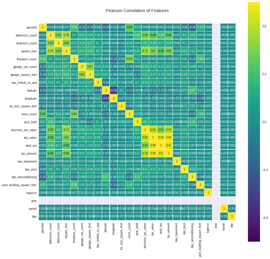
It’s also a good idea to scale the data at this point. I’ve left this out for brevity but you can refer to the full code if you are unsure how to do this.

Now a little preparation before we build our models. We’ll create an object called SklearnHelper that will extend the inbuilt methods (such as train, predict and fit) common to all the Sklearn classifiers. This cuts out redundancy as won’t need to write the same methods five times if we wanted to invoke five different classifiers.

# Class to extend the Sklearn classifier
class SklearnHelper(object):
    def __init__(self, clf, seed=0, params=None):
        params['random_state'] = seed
        self.clf = clf(**params)

    def train(self, x_train, y_train):
        self.clf.fit(x_train, y_train)

    def predict(self, x):
        return self.clf.predict(x)
    
    def fit(self,x,y):
        return self.clf.fit(x,y)
    
    def feature_importances(self,x,y):
        return(self.clf.fit(x,y).feature_importances_)

We’ll also define a function for Cross Validation. This deserves a little explanation. The function will be passed the model, the training set and the test set (for all six time periods). It will make kf=5 folds of the training data, train the model on each fold and make predictions for each time period using this model. It will then take an average of the predicted scores across the five folds for each time period.

def get_oof(clf, x_train, y_train, x_test_201610, x_test_201611, x_test_201612, x_test_201710, x_test_201711, x_test_201712):
    oof_train = np.zeros((ntrain,))
    
    oof_test_201610 = np.zeros((ntest,))
    oof_test_201611 = np.zeros((ntest,))
    oof_test_201612 = np.zeros((ntest,))
    oof_test_201710 = np.zeros((ntest,))    
    oof_test_201711 = np.zeros((ntest,))
    oof_test_201712 = np.zeros((ntest,))
    
    oof_test_skf_201610 = np.empty((NFOLDS, ntest))
    oof_test_skf_201611 = np.empty((NFOLDS, ntest))
    oof_test_skf_201612 = np.empty((NFOLDS, ntest))
    oof_test_skf_201710 = np.empty((NFOLDS, ntest))
    oof_test_skf_201711 = np.empty((NFOLDS, ntest))
    oof_test_skf_201712 = np.empty((NFOLDS, ntest))
    
    #train_index: indicies of training set
    #test_index: indicies of testing set
     
    for i, (train_index, test_index) in enumerate(kf):
        #break the dataset down into two sets, train and test
        x_tr = x_train[train_index]
        y_tr = y_train[train_index]
        x_te = x_train[test_index]
        
        clf.train(x_tr, y_tr)
        
        #make a predition on the test data subset
        oof_train[test_index] = clf.predict(x_te)
        
        #use the model trained on the first fold to make a prediction on the entire test data 
        oof_test_skf_201610[i, :] = clf.predict(x_test_201610)
        oof_test_skf_201611[i, :] = clf.predict(x_test_201611)
        oof_test_skf_201612[i, :] = clf.predict(x_test_201612)
        oof_test_skf_201710[i, :] = clf.predict(x_test_201710)
        oof_test_skf_201711[i, :] = clf.predict(x_test_201711)
        oof_test_skf_201712[i, :] = clf.predict(x_test_201712)
    
    #take an average of all of the folds
    oof_test_201610[:] = oof_test_skf_201610.mean(axis=0)
    oof_test_201611[:] = oof_test_skf_201611.mean(axis=0)
    oof_test_201612[:] = oof_test_skf_201612.mean(axis=0)
    oof_test_201710[:] = oof_test_skf_201710.mean(axis=0)
    oof_test_201711[:] = oof_test_skf_201711.mean(axis=0)
    oof_test_201712[:] = oof_test_skf_201712.mean(axis=0)
    
    return oof_train.reshape(-1, 1), oof_test_201610.reshape(-1, 1), oof_test_201611.reshape(-1, 1), oof_test_201612.reshape(-1, 1), oof_test_201710.reshape(-1, 1), oof_test_201711.reshape(-1, 1), oof_test_201712.reshape(-1, 1)

Next we’ll create a Dict data type to hold all of our model parameters.

SEED = 0 # for reproducibility
NFOLDS = 5 # set folds for out-of-fold prediction

# Put in our parameters for said classifiers
# Random Forest parameters
rf_params = {
    'n_jobs': -1,
    'n_estimators': 500,
     'warm_start': True, 
     #'max_features': 0.2,
    'max_depth': 6,
    'min_samples_leaf': 2,
    'max_features' : 'sqrt',
    'verbose': 0
}

# Extra Trees Parameters
et_params = {
    'n_jobs': -1,
    'n_estimators':500,
    #'max_features': 0.5,
    'max_depth': 8,
    'min_samples_leaf': 2,
    'verbose': 0
}

# AdaBoost parameters
ada_params = {
    'n_estimators': 400,
    'learning_rate' : 0.75
}

# Gradient Boosting parameters
gb_regressor_params = {
    'n_estimators':500, 
    'learning_rate':0.1,
    'max_depth':1, 
    'random_state':0, 
    'loss':'ls'
}

We’ll now create our models.

rf = SklearnHelper(clf=RandomForestRegressor, seed=SEED, params=rf_params)
et = SklearnHelper(clf=ExtraTreesRegressor, seed=SEED, params=et_params)
ada = SklearnHelper(clf=AdaBoostRegressor, seed=SEED, params=ada_params)
gb_regressor = SklearnHelper(clf=GradientBoostingRegressor, seed=SEED, params=gb_regressor_params)

And now train the models…

et_oof_train, et_oof_test_201610, et_oof_test_201611, et_oof_test_201612, et_oof_test_201710, et_oof_test_201711, et_oof_test_201712 = get_oof(et, x_train, y_train, x_test_201610, x_test_201611, x_test_201612, x_test_201710, x_test_201711, x_test_201712) # Extra Trees
rf_oof_train, rf_oof_test_201610, rf_oof_test_201611, rf_oof_test_201612, rf_oof_test_201710, rf_oof_test_201711, rf_oof_test_201712 = get_oof(rf,x_train, y_train, x_test_201610, x_test_201611, x_test_201612, x_test_201710, x_test_201711, x_test_201712) # Random Forest
ada_oof_train, ada_oof_test_201610, ada_oof_test_201611, ada_oof_test_201612, ada_oof_test_201710, ada_oof_test_201711, ada_oof_test_201712 = get_oof(ada, x_train, y_train, x_test_201610, x_test_201611, x_test_201612, x_test_201710, x_test_201711, x_test_201712) # AdaBoost
gb_regressor_oof_train, gb_regressor_oof_test_201610, gb_regressor_oof_test_201611, gb_regressor_oof_test_201612, gb_regressor_oof_test_201710, gb_regressor_oof_test_201711, gb_regressor_oof_test_201712 = get_oof(gb_regressor,x_train,y_train,x_test_201610, x_test_201611, x_test_201612, x_test_201710, x_test_201711, x_test_201712)

Finally, with the models trained, we have now reached the end of the first layer of our ensemble. We can now extract the features for further analysis.

rf_feature = rf.feature_importances(x_train,y_train)
print("rf_feature", rf_feature)
et_feature = et.feature_importances(x_train, y_train)
print("et_feature", et_feature)
ada_feature = ada.feature_importances(x_train, y_train)
print("ada_feature", ada_feature)
gb_regressor_feature = gb_regressor.feature_importances(x_train,y_train)
print("gb_regressor_feature", gb_regressor_feature)

The 23 features we obtain for each model are as follows:

rf_feature [ 0.04038533  0.02947441  0.14908661  0.0023588   0.00515421  0.01727217
  0.0020252   0.07555324  0.07418552  0.06010003  0.01318217  0.04547284
  0.11738776  0.09638334  0.07514663  0.11330465  0.00048846  0.00700142
  0.00589092  0.00323037  0.          0.03016362  0.03675231]
et_feature [ 0.06465583  0.0572915   0.12032578  0.00991171  0.01124228  0.00960876
  0.01485536  0.06740794  0.05175181  0.05436677  0.01772004  0.05594463
  0.09801529  0.0533328   0.0450343   0.08253611  0.00201233  0.02357432
  0.03032919  0.00296583  0.          0.061361    0.06575642]
ada_feature [  8.36785346e-03   3.79894667e-03   7.05391914e-02   7.82563418e-05
   3.22502690e-07   1.36595920e-02   0.00000000e+00   6.15640675e-02
   5.32715094e-02   3.73193212e-02   1.70693107e-02   1.18344505e-01
   1.72005440e-01   3.48224492e-02   4.48032666e-02   3.87885107e-02
   0.00000000e+00   7.54103834e-03   0.00000000e+00   1.06703836e-02
   0.00000000e+00   1.25617605e-01   1.81738430e-01]
gb_regressor_feature [ 0.02   0.012  0.246  0.     0.016  0.002  0.004  0.114  0.068  0.02
  0.004  0.012  0.158  0.056  0.06   0.16   0.     0.022  0.     0.     0.
  0.026  0.   ]

Let’s have a look at how important these features are for each model.

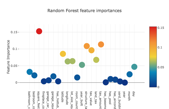
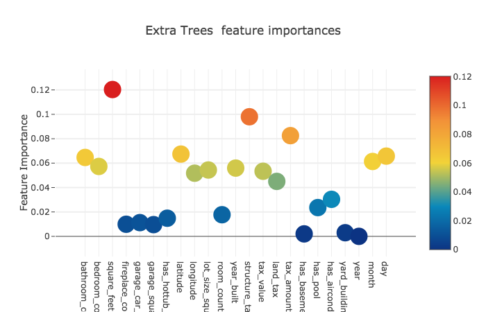
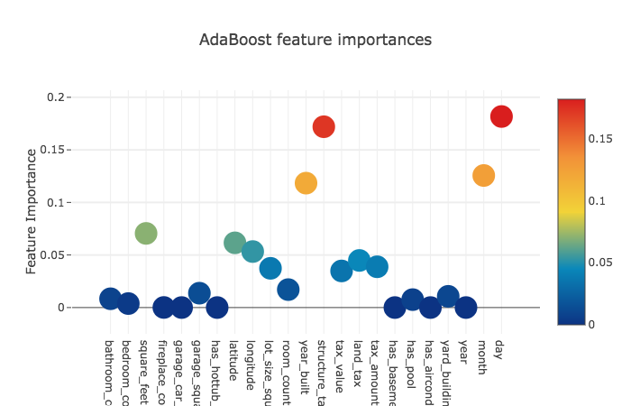
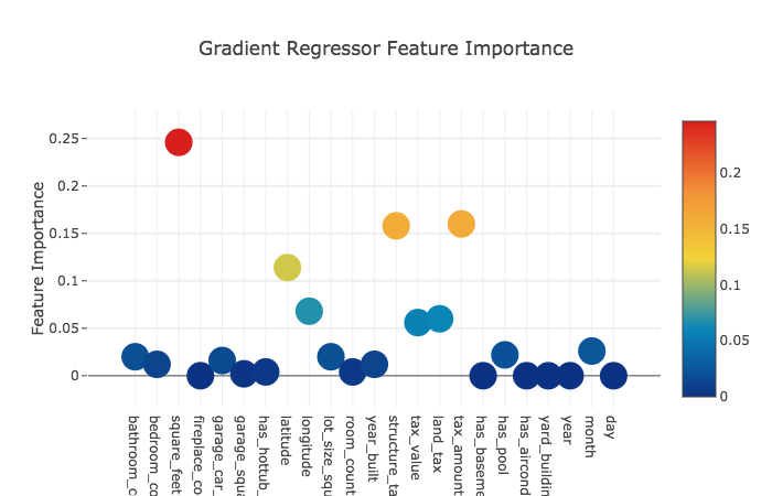
Now, across the four models, the mean feature importances.

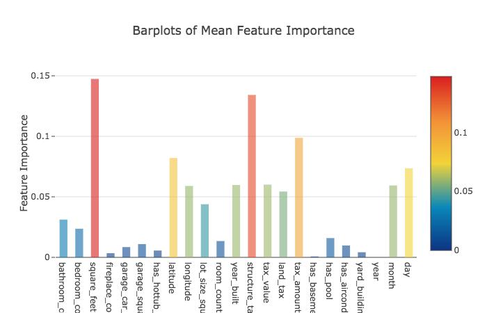
We can now build a new dataframe to hold these features, and train a regression model using xgboost on these features as our second layer.

#predictions from first layer become data input for second layer
base_predictions_train = pd.DataFrame( 
    {
    'RandomForest': rf_oof_train.ravel(),
    'ExtraTrees': et_oof_train.ravel(),
    'AdaBoost': ada_oof_train.ravel(),
    'GradientRegressor': gb_regressor_oof_train.ravel()
    })
#predictions for all instances in the training set
base_predictions_train.head(3)

gbm = xgb.XGBRegressor(
    #learning_rate = 0.02,
 n_estimators= 2000,
 max_depth= 4,
 min_child_weight= 2,
 #gamma=1,
 gamma=0.9,                        
 subsample=0.8,
 colsample_bytree=0.8,
 objective= 'reg:linear',
 nthread= -1,
 scale_pos_weight=1
 ).fit(x_train, y_train)

Now to make our final predictions…

predictions_201610 = gbm.predict(x_test_201610).round(4)
predictions_201611 = gbm.predict(x_test_201611).round(4)
predictions_201612 = gbm.predict(x_test_201612).round(4)

predictions_201710 = gbm.predict(x_test_201710).round(4)
predictions_201711 = gbm.predict(x_test_201711).round(4)
predictions_201712 = gbm.predict(x_test_201712).round(4)

StackingSubmission = pd.DataFrame({ '201610': predictions_201610, 
                                         '201611': predictions_201611,
                                         '201612': predictions_201612,
                                         '201710': predictions_201710,
                                         '201711': predictions_201711,
                                         '201712': predictions_201712,
                                         'ParcelId': ParcelID,
                            })
print(StackingSubmission)